Analysis of Corporate Finance

To fully understand this approach, you will need to read Analysis of Clinical Observations.

In large corporations it is easy to identify high-level problems, but finding out the root causes of these problems is more tricky.
Such corporations generate a deluge of information that can quickly drown anyone trying to analyze it.

For example, one of the principal measures of a company's performance is its final revenue. If the revenue shows a notable dip, then some analysis needs to be done to find out why. Such an analysis for Aroma Coffee Makers (ACM) showed that their equipment sales income was reduced, although their costs were still reasonable. This was most noticeable in their Northeast region. Looking further showed that their 1100 high-volume coffee maker family was well below its planned income, particularly in the government sector. Much of this is analysis of numbers, but further analysis may be more qualitative than quantitative. Perhaps this poor performance is due to a weak sales compensation plan, or government budget cuts, or a very hot summer, or strong competitor presence in the area.

All of this is much the same diagnostic process that is done by clinicians when investigating a patient's symptoms. From the obvious symptom we track back through likely causes, guided by our knowledge of the field. We hope to identify the root causes and then treat them. From this broad view of similar processes, we might hypothesize that we can apply the clinical models to corporate finance.

Clinical Observations gives a description of how qualitative and quantitative statements can be made about patients in a health care context.
That model can be applied to other contexts, such as analyzing corporate finances that looks at how this can be done.
The model works very well, but some modifications are required. Fortunately the patterns that describe these modifications are all extensions of the existing model rather than changes to it.

The first pattern replaces the person with some way of describing the segment of the enterprise under analysis. This Enterprise Segment (Section 1) describes a part of the enterprise defined along a series of dimensions. Each dimension represents some way of hierarchically breaking down the enterprise, such as location, product range, or market. The enterprise segment is a combination of these dimensions, a technique widely used by multidimensional databases.

The Measurement Protocol (Section 2) pattern describes how measurements can be calculated from other measurements using formulas that are instances of model types. Clinical Observations discusses how each measurement measures a phenomenon type; here we discuss how the measurement protocol defines ways of creating measurements for a particular phenomenon type. We cover three varieties of measurement protocols: Causal Measurement Protocols (Section 2.1) describe how different phenomenon types are combined to calculate another (sales revenue is the product of units sold and average price).
Comparative Measurement Protocols (Section 2.2) describe how a single phenomenon type can vary between Status Types (Section 2.3)
(actual versus plan deviation of sales revenue).
Dimension Combinations (Section 2.5) use the dimensions defined in the enterprise segment pattern to calculate summary values (calculate northeast sales revenue by totaling the values for individual states). Each of these sub types of measurement protocol uses polymorphism to determine its value.

Often we use qualitative phenomena to describe quantitative phenomenon types. In this case we can define the phenomena by linking them to a range of values for the phenomenon type. First we need a Range (Section 3), which allows us to describe a range between two quantities and various operations we want to do with the range. We can then define a Phenomenon With Range (Section 4) either by adding a range to the phenomenon using a Phenomenon With Range Attribute (Section 1) or by using a Range Function (Section 2).

We can combine the patterns examined in here with those in Clinical Observations to analyze a business' financial data.
Section 5 shows how we can use these patterns to identify the causes of problems in large corporations.

The models in this section are based on work done by a team from a large manufacturing company. This team explored using a health care model for corporate finance and found it to be a very useful foundation.

Key Concepts: Enterprise Segment, Dimension, Measurement Protocol, Status Type

1. Enterprise Segment

The most noticeable difference between the problem we examine in this section and the one discussed in Clinical Observations is that here not a single patient is being observed. In some cases we look at the whole company, but in other cases we observe only part of the company, such as 10-11 espresso sales to the government in the Northeast region. This could be handled by treating each part of the company, and the whole, as separate parties. However, it is important to ensure that the relationships between these corporate parts is understood.

Thus we have to alter the mapping from procedure to patient to point to some other type. This is an issue that we skimmed over in the discussion of mapping in Clinical Observations, so actually it is not such a problem as it may first appear. Clinical Observations approach does not actually link from observation to person.
In reality the link is to a type called object of care. Object of care is itself a generalization of patient and population. A population is a group of people and is used to allow observations to be made of groups of people, which is particularly important for public health.

For corporate finance we need a new sub-type of object of care, which we call enterprise segment, as shown in Figure 1. An enterprise segment is a part of a company, a part defined in a very particular way.

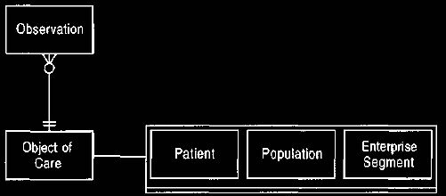
Figure 1 Object of care and its sub-types.
The patient of Clinical Observations is one kind of object of care that can be observed.

When we look at an enterprise, we can see that we can divide it into parts according to several criteria. It may be divided due to organizational unit, to geographical location, by product, by the industry sector that the product is being sold into, and so on. Each of these methods of division can be carried out more or less independently. Each can also be expressed as a hierarchy. For example, a multinational company can be divided first by market (USA), then by region (Northeast), then by area (New Hampshire). Each of these independent hierarchies is a dimension of the enterprise. New Hampshire and Northeast are elements at different levels in the geographical dimension. An enterprise segment is a combination of dimension elements, one for each dimension of the enterprise.
Thus the part of ACM that is northeast, 11 -10, government can be defined as the enterprise segment with dimension elements of
northeast on the geographical dimension, 11-10 on the product dimension, and government on the industry dimension, as shown in Figure 2. This approach to analysis, often referred to as a star schema, is commonly used in multidimensional databases.


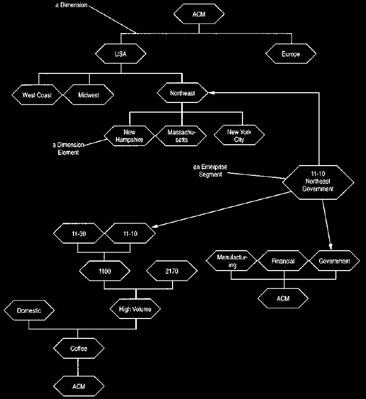
Figure 2 How enterprise segments link to elements in dimensions.
One enterprise segment is a combination of elements from each dimension.

With this enterprise segment defined, we can form a model of the relationships between the various types, as shown in Figure 3. We can link
dimension elements together into hierarchies. Many hierarchies of dimension elements can be defined. Note how the hierarchies constraint on the parent association is necessary because the cardinalities alone do not enforce a hierarchy (although they might allow cycles). The enterprise segment must have one element from each of these hierarchies, as indicated by the three associations from the enterprise segment. The constraint on the dimension element ensures that the hierarchies are all within the same dimension. The model will handle the situation quite well, but it has a couple of disadvantages. First, the concepts of dimension and dimension level are not properly defined, although they can be derived. Second, adding a new dimension will cause a model change.

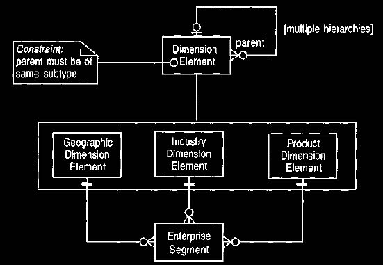
Figure 3 Defining enterprise segments with dimension elements.
Using this model requires adding a new sub-type whenever a dimension is added.

The model shown in Figure 4 uses an explicit dimension type. Each dimension holds a hierarchy of dimension elements. The enterprise segment then needs to have one link to a dimension element in each dimension. We can do this by using the keyed mapping. When combined with cardinality this mapping states that for each instance of the key (dimension) there is one and only one dimension element.

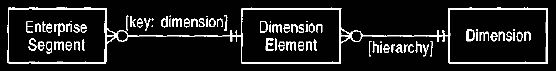
Figure 4 Defining enterprise segments by using dimensions and dimension elements.
This model allows us to add new dimensions without changing the model. It is also
more compact.

Example We can define the 11-10, Northeast government enterprise segment, linking it to the dimension elements 11-10, Northeast, and government.
11-10 is in the product dimension. Northeast is in the location dimension, and government is in the industry dimension.

Note that each hierarchy needs a top, and this does not necessarily show a named thing. A common convention is to label the top "all," showing that any segment that references it does not have any breakdowns along that dimension. Another convention would be to let the mapping to the dimension element be optional; then "nil" would indicate the top of the tree. The former approach is more consistent, despite this slightly artificial top element.

Example: If we add a channel dimension, then the enterprise segment 11-10 Northeast government has a link to the top dimension element of the channel hierarchy. We call this dimension element all.

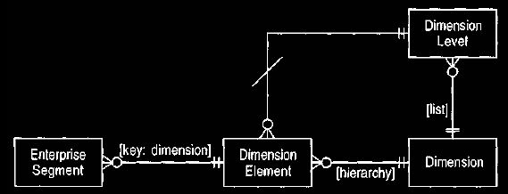
Figure 5 Adding dimension levels to Figure
Dimension levels allow us to name each level of a dimension.

Adding a type for dimension level is not entirely obvious. Naturally every dimension element has a dimension level. However, the level is determined by its position in the dimension's hierarchy. The model shown in Figure 5 deals with this by assigning each dimension a list to define its dimension elements. The dimension element uses its level in the hierarchy and the list of dimension levels to determine its dimension level.

Example In the ACM example the location dimension has a list of dimension levels: market, region, and area. New Hampshire is defined in the hierarchy with parent Northeast, whose parent is USA, whose parent is all. Since it is three levels down. New Hampshire's dimension level is the third in the list: area.

1.1 Defining the Dimensions

How can we define dimensions? The simplest definition is that they are the ways in which a large organization can be broken down via some organizational structure. However, that is not generally the most satisfactory definition. An organization can be broken down in many ways, depending on the situation.
In addition, some dimensions are not necessarily appropriate to an organization system. The model in Figure 2 includes a breakdown by industry to which ACM sells, but this need not represent an organization structure within ACM.

We can find a better way to define dimensions by looking at the bottom of the hierarchy and asking what is being classified by the dimensions there. In the example we can see that ACM is focusing on the sale or rental of a coffee machine. We can classify this dimension according to which machine was sold, which sales area sold it, and which industry it was sold into. The dimensions come from the classification of this focal event, which is the fact table of a star schema.

In determining the dimensions to use in this kind of analysis, first we need to understand what the focal event is. We can then look at the ways in which this focal event can be classified. From Figure 2 we see the focal event involves a product that has a product family, which has a product group, which has a beverage. On the sales dimension we see area, region, and market.

These dimensions and levels should be defined by business analysts; Figure 6 shows a good way to do this. As Figure 6 indicates this structure can become quite complex. The dimensions are not necessarily completely independent. For example, note how the price range dimension intersects the product dimension. This indicates that any product will have one particular parent along the product and price range dimensions. The model of Figure 5 would need to be modified to take this into account properly, although it is questionable whether it is worth undertaking this since it does complicate the model somewhat. This issue could be handled by the dimension creation process.

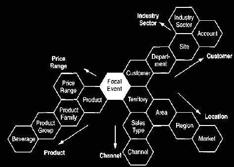
Figure 6: A Tilak chart showing a typical set of dimensions and levels.
This is a useful diagram providing we do not have more than six branches from any level.
In practice we rarely do.

The dimensions need not be measurable to the lowest level. In this case it might not be worthwhile, or even possible, to analyze down to an individual salesperson's territory or to an individual customer. In this case the dimensions are elaborated part of the way down to the underlying event. It is still useful to understand what the lower levels are, both for future development and to see the foundations of the higher levels.

A full analysis of the customer's domain would involve producing a business model for the customer's area. This would include a structural model, which would be used to rigorously define the dimensions. Each dimension should represent a hierarchical path along the structural model. The details of this process are beyond the scope of this section. For the sake of discussion we will assume the dimensions have been determined.

The dimensions can be defined explicitly by the user of the analysis system. Otherwise, they can be determined from corporate databases. For the latter, each dimension needs a builder operation to tell it how to query corporate databases. This allows the system to add nodes to the dimension over time.

1.2 Properties of Dimensions and Enterprise Segments

An important rule about dimensions is that the measurements for dimensions at lower levels can be properly combined into the higher level. Thus if we want to look at sales revenue for the Northeast, we can do this by adding together the values for sales for all sub-regions of the Northeast region.

Any dimensions that are defined must support this property. Usually dimensions are combined through addition, but there are some exceptions.

Along with dimensions defined through business structures, another common dimension is time. Time is treated as a dimension by classifying the underlying event into a time period. If these periods are months then we can talk about such figures as revenue for (11-10, Northeast, March 2004).
This implies a dimension element for March 1994 that would be a child of the dimension element for 199 The time dimension satisfies the combinability property discussed above, providing the figures are only for that month (and not year-to-date figures). We can easily calculate year-to-dates from month-only figures but typically not by combining along a dimension.

Enterprise segments share an interesting property with more fundamental types: All enterprise segments conceptually exist. There is no notion of conceptually creating the number 5, the quantity $5, or the date 1/1/2314. These things all exist in our minds but may need to be created as objects in the computer.
Enterprise segments share this property. Once all dimensions have been specified with their dimension elements, then all enterprise segments conceptually exist, although they may not be created as software objects.

This shared property raises the question of whether an enterprise segment should be treated as a fundamental type. If so, it should not
have any mappings to non-fundamental objects. A dimension element and an observation (inherited from an object of care) are both non -fundamental.
Although the latter could be excluded, the former is part of the definition of enterprise segment and thus cannot be excluded. There is also a lot of sense in holding the mapping from an enterprise segment to an observation since a very common request is to find all observations for a given enterprise segment. In balance it seems that enterprise segments are not fundamental, despite this property of universal conceptual existence.

Treating enterprise segments as non-fundamental does have an effect on the interface. The create operation is really a find-or-create. It first looks to see if the required instance of the enterprise segment exists; if so it returns it, if not it creates it. (Or you can think of it as not having a create operation but only a find operation, which creates silently when it needs to.)

2. Measurement Protocol

The corporate analysis we have been discussing uses a lot of measurements. These measurements are not entered by hand; usually they are either loaded from one of many databases or calculated from other measurements. We need to remember how we can make these measurements, that is, the protocol we use to create the measurement. Figure 7 shows a general outline of measurement and protocols, much of it similar to that of Clinical Observations.

Two kinds of measurement protocol are shown in Figure 7. Source measurement protocols refer to queries against some corporate database. Typically an object knows logically which database it is accessing, although the actual commands are in another layer. The user should decide which data base is accessed. A calculated measurement protocol represents a calculation done on measurements already present in this domain.

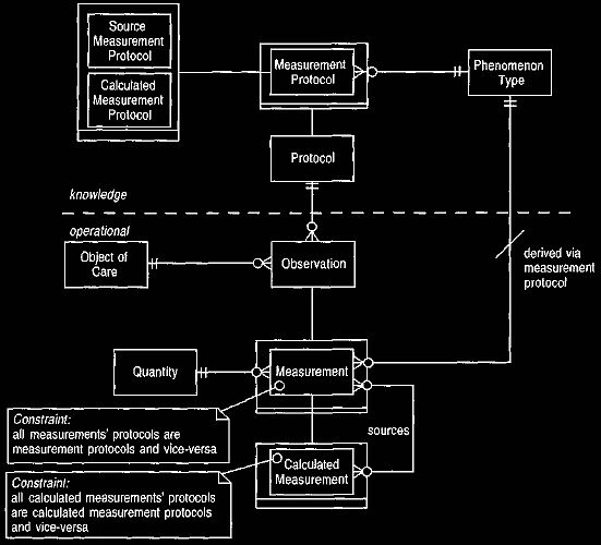
Figure 7 Measurement and measurement protocols.
Source measurements are from a database, and calculated measurements use
formulas.

An important point about this model --a reflection of its clinical back-ground - is that any phenomenon type can have several measurement protocols to determine its value. This point may strike some readers as odd. What is the point of a measurement that we can calculate in more than one way? If there is more than one formula, surely it is a different phenomenon type. The first and most obvious point is that the phenomenon type can have both calculations and source protocols. We can use different protocols at different times. There can also be multiple source protocols; which one we use depends on system availability.
Some databases are more reliable than others, but availability can never be perfect.

Similarly the user could consider using different calculations to produce the same phenomenon type. Which calculation the user chooses can depend on which sources are available or on the user's opinion about subtle points within the calculation. A good example of this is the value of inventory. Usually inventory is physically counted only at the end of the year, but its value needs to be estimated at other times. In either case the value is used in the same way for further financial information.

Some users of this model may choose to specify which measurement protocol to use to come up with a value. Others, however, may just want a phenomenon type and leave it to the system to come up with how it gets it. In the latter case some way is needed to prioritize the measurement protocols for a phenomenon type. This can be done by making the mapping from phenomenon type to measurement protocol a list. The front of the list defines the preferred protocol and so on.

Note the presence of calculated measurement, with its link back to its source measurements. This follows the general rule that the result of a computation, when treated as an object, should know what computation caused it (the protocol) and what the inputs to this protocol were (the sources).

2.1 Holding the Calculations

The calculated measurement protocols include the formulas by which they are calculated, as shown in Figure 8. This is an example of an individual instance method (see Analysis of Inventory and Accounting, Section 6). The formulas for calculated measurement protocols are often very simple, so we can use a simple interpreter pattern and hold the formulas as spreadsheet-style formulas.

An important feature of the model is the way the arguments are presented. Each calculated measurement protocol has a list of arguments. This list represents those phenomenon types that are combined in the formula. Note that the mapping is a list. For the formula to make sense, the elements in the mapping must be identifiable. A list is a good way to do this. Alternatively they can be keyed by a string.

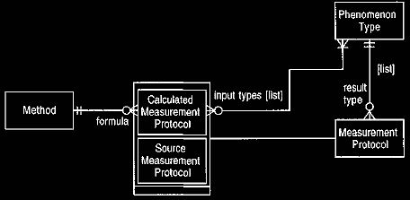
Figure 8 Methods for calculated measurement protocols.

Example: Sales revenue is a phenomenon type with a causal calculation as its measurement protocol. The arguments to the causal calculation are a list of two phenomenon types--number of sales and average price. The method is the formula arg[1]*arg[2].

Example Body mass index is a phenomenon type in medicine. It has a causal calculation with arguments of weight and height. The method is the formula weight/height.

2.2 Comparative and Causal Measurements Protocols

In a corporate finance application the measurements are not absolute values. The users are usually not too interested in a figure that says revenues are $x, rather they are interested in the difference between the actual and a planned figure or this year's revenues compared to last year's.

To consider these comparative measurements, we need to describe the various kinds of measurements that can appear. Typical comparisons are between an actual value and either a prior or a planned value. Prior values can be considered by either looking at the applicability time reference (see Clinical Observations, Section 8) or by looking for a measurement for the enterprise segment that has a prior time dimension. Planned measurements require us to make a distinction between actual or planned values, which correspond to the active and projected observations discussed in Section 3.10. In addition, the projected observation must record what plan was the source for the projection, so that we can distinguish between annual plans, quarterly forecasts, and the like, as shown in Figure 9.

At this point a fundamental distinction between two types of calculation should be apparent. One kind is determining a value for a phenomenon type based on values of other phenomenon types. For example, we can calculate sales revenue by multiplying the number of sales by the average price. This type of calculation is called a causal calculation because it follows the cause and effect analysis. Causal calculations can have any number and any relationship of input phenomenon types, and the formulas by which they are computed can be any expression.

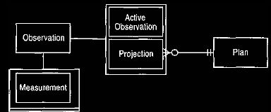
Figure 9 Kinds of observations to support planned and actual values.

Comparative calculations, on the other hand, are more structured. They always have two input measurements, which must be of the same phenomenon type. The output measurement's phenomenon type is always derived from the form of the calculation and the input phenomenon type. Thus if we are looking at the deviation of number of sales, then the inputs will be the phenomenon type number of sales and the output phenomenon type will be deviation for number of sales. The formulas for these calculations will generally be of a fairly limited set: such things as absolute deviation (x-y) or percentage deviation ((x-y)/y).

The differences between these two types of calculations can be formalized by sub-typing the calculated measurement protocol, as shown in Figure 10. The calculated measurement protocol carries the key elements of the structure. Each calculated measurement protocol has a single result type and a number of input types. For comparative calculations they are limited to two arguments, which must be the same phenomenon type. All calculated measurement protocols have a method that contains the formula by which a new value is calculated from the inputs. Two protocols can share a single method, for example the method arg1 - arg2 is shared between all the protocols that determine absolute deviation for all the phenomenon types. Indeed, this case is so common it is worth making a special sub-type for it that fixes the method to the type.

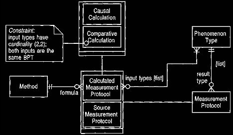
Figure 10 Types of calculation as shown by calculated measurement protocols.
Causal calculations link different phenomenon types, and comparative calculations show
the difference in one phenomenon type between status types.

2.3 Status Type: Defining Planned and Actual Status

Measurements determined by source or calculated measurement protocols are always calculated through their measurement protocol. The measurement protocol provides a factory method for the measurement. (Note that the reason for this is that the method of creation varies, rather than the type of the final result. This is another reason to use the factory method.)

A client asks the measurement protocol to create a measurement. The client needs to tell the measurement protocol what object of care it needs to reference. The client also needs to tell the protocol whether it is an actual or planned value: which plan for the planned value or which date for the actual value.

At this point the model shown in Figure 9 shows a weakness. There is no simple way we can provide the information needed for the protocol. Figure 9 does provide a good way to determine this information from an existing measurement, but it does not provide a convenient single way to ask for the information. This can be overcome by the model shown in Figure 11, which puts these properties together into a single status type. Two sub-types exist of the abstract status type. Actual status types may have a time offset. For current values there will be no offset (or it can be zero). Six months or one year ago will have the appropriate offset. Planned status types have the appropriate plan, just like projections.

Example A corporation assesses four kinds of financials: actual value, prior year, the annual plan, and the latest quarterly forecast. The actual would be an actual status type with time offset of zero. The prior year is an actual with time offset of one year. The annual plan is a planned status type linked to the annual plan. The quarterly fore cast is also a planned status type linked to the latest quarterly forecast. All the quarterly forecasts are instances of the plan.

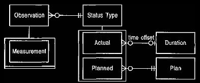
Figure 11 Status types as an alternative to Figure 9.
This alternative makes it easier to specify the kind of comparative measurement
required (see Figure 12).

Effectively we have moved the knowledge of what kind of observation we have from the observation itself to a separate type. This type can enumerate all possible variations independently of existing observations. The type resides at the knowledge level so we can calculate new measurements, but it need not be at the knowledge level.
We should note that this is not inconsistent with the model in Figure 9. Both expressions say the same thing, in slightly different ways,
and both could be supported at the same time.

Now the client needs only to specify the status type for the measurement protocol to have enough information to create the measurement, assuming the protocol is a causal protocol. Comparative calculations need two status types, one for each input. One way of dealing with this is to vary the create measurement operation so that it requires one status type for causals and two for comparative measurements. Another method is to allow comparative status types, as shown in Figure 12. The latter method is preferable because the comparison is now an object in its own right, and the interface for creating all measurements is the same.

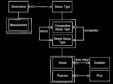
Figure 12 Using comparative status types to ease the specification of comparative measurements.

Example ACM management wants to see the actual vs. planned deviation for sales revenue. To satisfy this request, the model must include a phenomenon type for sales revenue and a phenomenon type for sales revenue deviation. The sales revenue deviation is a comparative calculation with a method of arg[1] -arg[2].The request creates an observation of sales revenue deviation with a comparative status type. The status type will have datum of planned and comparator of actual.

2.4 Creating a Measurement

Now that we know how to ask for a new measurement, we can look at the process for creating a measurement, which is illustrated in Figures 13 and 14. The process has three steps: finding the arguments, executing a formula, and creating a new measurement object with the resulting value.

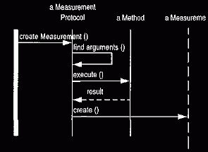
Figure 13 Interaction diagram for creating a measurement.

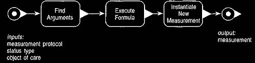
Figure 14 Event diagram that describes the process for creating a measurement.

The argument-finding operation is polymorphic depending on whether we have a causal or comparative measurement protocol. The causal protocol, shown in Figure 15, needs to find all measurements of the same status type and object of care whose phenomenon types match the input types of the protocol.
The comparative formula, shown in Figure 16, looks for two measurements whose phenomenon type is that of the input type, who have the same object of care, and whose status types are the datum and comparator for the protocol.

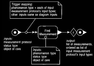
Figure 15 The find arguments operation for a causal calculation.
This operation finds a measurement for each argument type with all other factors the
same.

When we have found the arguments, we can pass them on to the formula and then create a measurement with the resulting value.

2.5 Dimension Combinations

A third kind of calculation is the combination of values along a dimension. The example mentioned above was that of calculating sales revenue for the Northeast by adding together the values for sales for all child regions of the Northeast region. More precisely, the measurement of a phenomenon type for an enterprise segment that refers to Northeast is calculated by finding all measurements of that phenomenon type attached to enterprise segments that refer to child regions of the Northeast dimension element but have the same dimension elements along the other dimensions. These values are added together for the new value.

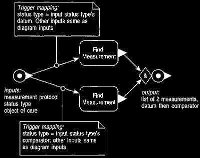
Figure 16 The find arguments operation for comparative calculations.
This operation finds one argument for each leg of the comparative status type.

We can thus add a dimension combination protocol as shown in Figure 17.

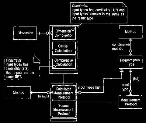
Figure 17 Adding dimension combination to the calculated measurement protocols.

We must specify the dimension that is being combined. The calculation does not need any input types (since it is always the same phenomenon type as the output type). We could consider reducing the input type mapping's cardinality to zero, but we think we can preserve the sense better by keeping the mapping mandatory and adding a constraint. Creating the measurement follows the usual steps shown in Figure 14, with the find arguments operation again being altered as in Figure 18.

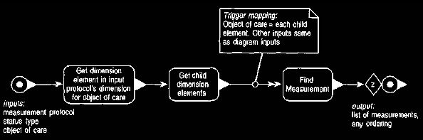
Figure 18 The find arguments operation for dimension combination calculations.
This operation finds a measurement for each child enterprise segment along the indicated dimension.

The role of the calculation method is very simple: It takes all the arguments and adds them together. Usually addition is used for combining, but not always. For example, the phenomenon type average price is not added in dimension combination; instead a mean is found. These variations depend on the phenomenon type, so each phenomenon type needs to have a combination method. The calculation method applies the combination method to the arguments to determine the result.

Note that the comparative and dimension combination protocols can be automatically generated. For dimension combination, one protocol can be defined for each combination of phenomenon type and dimension. For comparative calculations, one protocol can be defined for each combination of phenomenon type and kind of comparative calculation.

Calculated measurements are just as useful in health care. We discuss calculated measurements in this section, rather than in Clinical Observations, primarily because they were used extensively in our work on corporate finance. Thus they are an illustration of how taking a model to a different domain causes more thought that may well feed back into the original domain.

So far we have looked at how we can use measurements, both calculated and sourced, to investigate a company's financial performance. The measurement protocol pattern gives us a way of looking at this information quantitatively. To make sense of a forest of numbers, however, it is often useful to group measurements into categories. We might want to divide the absolute revenues into a number of bands, or we could highlight as problems all comparative measurements that are 10 percent below the datum.

Our first step is to describe ranges of measurements, which is the subject of this pattern. The second step is to link these ranges into the broader system of observations, as we will discuss in Section 4. We often come across the need to hold a range of some values. The range can consist of numbers (such as 1..10), dates (such as 1/1/95..5/5/95), quantities (such as 10..20kg) or even strings (such as AAA..AGZ).
Usually a range is placed on the type that is using it by giving that type separate mapping for an upper and lower value, as shown in Figure 19.

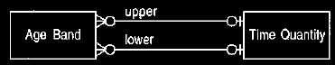
Figure 19 Representing a range with upper and lower bounds on the type that uses it.
We do not recommend this approach to ranges; use a range type instead.

The problem with this approach is that there is rather more to ranges than just an upper and lower value. We might want to know whether a particular value is within a range, whether two ranges overlap, whether two ranges abut, or whether a set of ranges form a continuous range. Such behavior would have to be copied for every type that has upper and lower values. The solution is to make the range an object in its own right, as shown in Figure 20. In this situation all responsibilities which are essentially about ranges are contained within the range, and do not need to be duplicated in those types that use ranges.

In general a range can be formed between any two magnitudes. A magnitude, in essence, is a type that defines the comparative operators (>, <, =, >, <).

3. Range

The range needs only these operations to define its own key operations: includes, overlaps, and abuts. When a range is used, the using type usually indicates what kind of magnitudes it wants in its range. There are several ways of modeling which kind of magnitude is required. One way is to declare a sub-type, such as we do with time period (a range whose magnitudes are time-points). Another way is to
use a constraint, as in Figure 20. A third way is to use something along the lines of parameterized classes, where a range of integers is defined by a type called range<Integer>. Conceptually all of these modeling techniques are equivalent, so
we can use whatever we find the easiest. In implementation we need to choose more carefully, and the trade-offs vary depending on the implementation environment. The choice of conceptual model does not imply anything about the implementation.

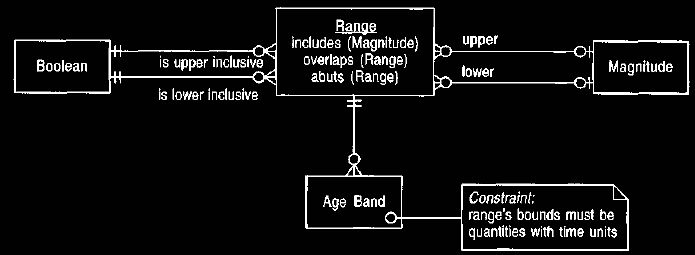
Figure 20 Using an explicit range object.
This should always be done when an upper and lower value are needed. Upper and lower mappings are optional, thus allowing open-ended ranges, such as less than 6 months.
The Booleans are needed to differentiate less than 6 months from less than or equal to 6 months.

4. Phenomenon with Range

Ranges give us a way to define categories of measurements. We now need to link them into the broader model of observation and measurement. To do this, we can form phenomena of certain phenomenon types. If our phenomenon type is revenue percentage deviation, we can form a phenomenon of revenue problem, which exists when our revenue percentage deviation is less than -10 percent. This implies that a measurement of-12 percent of revenue percentage deviation also implies a category observation of revenue problem.
The first question we need to answer is whether there are one or two observations. According to the model shown in Figure 3.9, observations are either measurements or category observations, they cannot be both. We can allow a single observation to be both by using the model shown in Figure 21. The choice between the models depends on whether we consider the conceptual process as being first a measurement and then a separate step of observing the revenue problem, or whether we see the measurement and observation as one process. For simple cases such as these, the domain experts we have worked with preferred the latter.

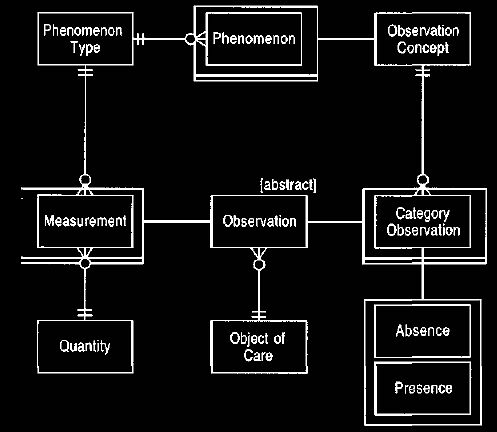
Figure 21 Allowing an observation to be both a measurement and a category observation.
The [abstract] statement implies that an observation must be at least one of its sub-types.

Since we have a well-defined range, it seems natural to let the computer automatically link any such measurement to the relevant phenomenon. To do this we need a way of defining the range within the knowledge level.

4.1 Phenomenon with Range Attribute

The simplest approach is to add a range to a phenomenon, as shown in Figures 22 and 23. Then when we create a measurement we can look to see if it falls in the range for any phenomenon of that measurement's phenomenon types. We do have to consider whether we want the range for a phenomenon type not to overlap or to be complete. Either of these conditions indicate the need for a constraint.

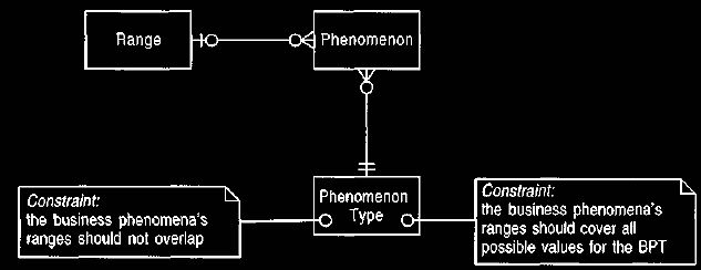
Figure 22 Adding a range to a phenomenon

The measurement protocol creates a measurement. It asks its phenomenon type for its phenomena. It asks each phenomenon if it includes the new measurement. If so, it classifies the measurement as a category observation of the BP.

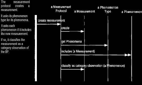
Figure 23 Interaction diagram for creating a measurement and checking the phenomena.
The responsibility for checking the phenomena could be done equally well by the measurement object.
We prefer the protocol, as we think that is a more likely place for overriding.

Example Revenue percentage deviation is divided into four categories: greater than 5% is good, 5% to -5% is OK, -5% to -10% is warning, and less than -10% is a problem.
This can be represented as four phenomena for the phenomenon type revenue percentage deviation (RPD). The phenomenon good RPD has a range with no upper bound and 5 lower bound, the phenomenon OK RPD has a range with upper bound 5 and lower bound -5, the phenomenon warning RPD has a range with upper bound -5 and lower bound -10, the phenomenon problem RPD has a range with upper bound -10 and no lower bound.
It is important to check exactly what the boundaries are and include this information in the ranges; so we ask if exactly 5% is good RPD or OK RPD?

Example Body mass index is used to define four groups: normal 20-25 kg/m2, overweight 25-30 kg/m2, obese 30-40 kg/m2, morbid obese >40 kg/m2.
This would be represented as four phenomena for the phenomenon type body mass index. The overweight phenomenon would have a range with lower bound 25 kg/m2,and upper bound 30 kg/m2. Each of the other phenomena would have similar ranges.

4.2 Range Function

An alternative approach is to create a separate range function as a sub-type of associative function, as shown in Figures 24 and 25. This is useful when different ranges apply, depending on the context described by an observation concept. This model allows several series of ranges to be present, depending on which observation concepts apply. The range function evaluates some expression of the arguments, as in an associative function, but also checks whether the measurement falls in the range over a phenomenon type. If both are true, then the product observation concept applies.
Developing constraints to ensure that only one range function will be true for any given measurement is considerably more difficult than when ranges are applied directly to phenomena.

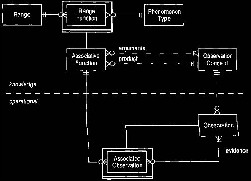
Figure 24 Range function.


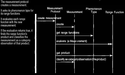
Figure 25: Creating a measurement and checking range functions.
The measurement protocol creates a measurement. It asks its phenomenon type for its range functions. It evaluates each range function with the new measurement. If the evaluation returns true, it finds the range function's product and classifies the measurement as a category observation of that product.

Example Certain enterprise segments are defined as key. For these segments the problem revenue percentage deviation (RPD) is defined at -5% instead of -10%.
To handle this we would define an observation concept of key segment. Those segments that were key segments would have an appropriate observation applied to them.
(This would also give us the ability to change key status over time.) We would define a range function with arguments of {key segment}, product of problem RPD, a range of <5% and a phenomenon type of RPD.

Example The normal range of a person's beta HCG increases with pregnancy. To represent this, we would have two range functions with the product normal beta HCG.
One would have arguments of pregnancy and the other arguments of nonpregnancy. The phenomenon type on the range functions would be beta HCG.

Both of these approaches have their merits, and it can be plausible to use them both together. Linking directly to the phenomenon is certainly the easiest way of doing it, and that is the one to use if it correctly describes the situation. Range functions are more complex but can represent more complicated situations.
So you should use the direct link to phenomenon when you can and range functions when you must. If the situation gets more complex than the models described here can handle, you should add features to range function, either directly or by way of a sub-type.

5. Using the Resulting Framework

So far this section has described patterns that represented expansions of those introduced in Clinical Observations.
Now we can look at how we can use these models.

We begin by looking for the total revenue for ACM. This would be a measurement whose enterprise segment is the whole company; that is, the enterprise segment's dimension elements are all at the top of the dimension hierarchies. The measurement normally would not be an absolute value; rather it would be a comparative value with some plan or prior time period. Furthermore, the fact that it is a problem might be indicated by highlighting it according to a ranged phenomenon. The analyst would then begin by looking for problem observations defined by phenomena.

To identify that the problem is with equipment sales income, we need to roll back the causal calculation of total revenue as sales income minus sales cost. Note that the causal calculation indicates a possible path of analysis, whether or not the measurement was determined that way. It may be that this final figure was actually sourced from a database. (Due to dirty data, it may be that it doesn't exactly fit the result of the formula.)

The next step is to use dimension combination protocols. Looking along the location dimension shows that the Northeast segment had a noticeably higher deviation. We can now focus on the enterprise segment that points to the Northeast dimension element on the location dimension, and at the top for all other dimensions. Repeating this process two more times would lead us to the enterprise segment with location of Northeast, product of 1100 family, and industry sector of government.

There is a certain amount of indirection here. When comparative calculations are involved, the route may not be direct. It may not be that the deviation in total revenue is calculated by subtracting the deviation in sales cost from the deviation in sales income. A more likely scenario is that the separate actual and planned sales revenues are calculated, and then these are used in the causal. With absolute deviation, either route will work, but this is not true for percentage deviation. The presence or absence of protocols will indicate what will and will not be appropriate calculations.

We can use alternative routes. Instead of first doing the causal, and then dimension combinations, we could break down on the location dimension, then use a causal, and then other dimension breakdowns. There are many possible paths for analysis, and these need not be the same as those used for calculating the figures.

We can describe qualitative statements, such as "a strong competitor may cause a decrease in sales," using the associative functions described in Clinical Observations. Section 11. Qualitative and quantitative observations are linked by assigning ranged phenomena.