Analysis of Observations and Measurements in Clinical, Medical, and Pharmaceutical Business

Observations and Measurements

Many computer systems record information about objects in the real world. This information finds its way into computer systems as records, attributes, objects, and various other representations. The typical route is to record a piece of information as an attribute to an object. For example, the fact that a person weighs 185 pounds would be recorded in an attribute of a Person type.
This page examines how this approach fails and suggests more sophisticated approaches.

We begin by discussing Quantity (Section 1) - a type that combines a number with the unit that is associated with it. By combining numbers and units, we are able to model the world more exactly. With quantities and their units modeled as objects, we can also describe how to convert quantities with a Conversion Ratio (Section 2).
The quantity pattern can be extended by using Compound Units (Section 3), which represent complex units explicitly in terms of their components.
Quantities are required for almost all computer systems; monetary values should always be represented using this pattern.

Quantities can be used as attributes of objects to record information about them. This approach begins to break down, however, when there is a very large number of attributes that can bloat the type with attributes and operations. In these situations Measurement (Section 4) can be used to treat measurements as objects in their own right. This pattern is also useful when you need to keep information about individual measurements. Here we begin to see the use of operational and knowledge levels on this page.

Measurements allow us to record quantitative information. Observation (Section 5) extends this pattern to deal with qualitative information and thus allows Sub-typing Observation Concepts (Section 6) in the knowledge level. It is also often essential to record the Protocol (Section 7) for an observation so that clinicians can better interpret the observation as well as determine the accuracy and sensitivity of the observation.

A number of small patterns extend observation. The difference between the time an observation occurred and when it is recorded can be captured with a Dual Time Record (Section 8). Often it is important to keep a record of observations that have been found to be incorrect; this requires a Rejected Observation (Section 9). The biggest headache with observation is dealing with certainty, for it is often important to record hypotheses about objects. The sub-typing of Active Observation, Hypothesis, and Projection (Section 10) is one way of dealing with this problem.

Many statements about observations are made using a process of diagnosis.

We infer observations based on other observations. Associated Observation (Section 11) can be used to record the evidence observations, plus the knowledge that was used for the diagnosis.

The preceding patterns are structural and are used to make records of our observations. To understand how they work, it is useful to consider the Process of Observation (Section 12), which can be modeled with an event-based technique.

Few professions have such complex demands on measurements and observations as medicine.
The ideas here can be transplanted to other areas: see Analysis of Corporate Finance page.

Key Concepts

Quantity, Unit, Measurement, Observation, Observation, Concept, Phenomenon Type, Associative Function, Rejected Observation, Hypothesis.

The simplest and most common way of recording measurements in current computer systems is to record a number in a field designed for a particular measurement, such as the arrangement shown in Figure 1. One problem with this method is that using a number to represent a person's height is not very appropriate. What does it mean to say that someone's height is 6, or that someone's weight is 185?

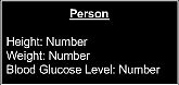
Figure 1 Number attribute.
This approach does not specify the units.

To make sense of the number, we need units. One way of doing this is to introduce a unit into the name of the association (for example, weight in pounds). The unit clarifies the meaning of the number, but the representation remains awkward. Another problem with this technique is that the recorder must use the correct units for the information. If someone tells us their weight is 80 kilograms, what am we to record? Ideally a good record, especially in medicine, records exactly what was measured--no more, no less. A conversion, however deterministic, does not follow that faithfully.

In this context a very useful concept is that of quantity. Figure 2 shows an object type that combines number and units, for example, 6 feet or 180 pounds. Quantity includes appropriate arithmetical and comparative operations. For example, an addition operation allows quantities to be added together as easily as numbers but checks the units so that 34 inches are not added to 68 kilograms. Quantity is a "whole value" [2] that the user interface can interpret and display (a simple print operation can show the number and the unit). In this way quantity soon becomes as useful and as widely used an attribute as integer or date.

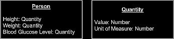
Figure 2 Measurements as attributes using quantity.
Quantity should always be used where units are required.

Example: We can represent a weight of 185 pounds as a quantity with Value of 185 and Unit of pounds.

Monetary values should also be represented as quantities (we can use the type money), using a currency as the unit. With quantities you can easily deal with multiple currencies, rather than being tied to a single currency.
Money objects can also control the representation of the amount.
Often rounding problems occur in financial systems if floating point numbers are used to represent monetary values; monetary quantities can enforce the use of fixed point numbers for the Value attribute.

The use of quantity is an important feature of object-oriented analysis. Many modeling approaches make a distinction between attributes and associations.
Associations link types in the model, and attributes contain some value according to some attribute type. The question is, what makes something an attribute rather than an association? Usually attributes are the typical built-in types of most software environments (integer, real, string, date, and so on. Types such as quantity do not fit into this way of choosing between attribute and association.

Some modellers say quantity should be modeled with an association (because it is not a typical built-in type), while other modellers recommend an attribute (because it is a self-contained, widely used type). In conceptual modeling it doesn't really matter which way you do it, the important thing is that you look for and use types such as quantity. Since we don't distinguish between attributes and mappings, we don't get into this argument.
(We are laboring this point because we find types such as quantity conspicuously absent from most of the models we see.)

2. Conversion Ratio

We can make good use of units represented explicitly in the model. The first service that units can perform is to allow us to convert quantities from one unit to another. As shown in Figure 3 we can use conversion ratio objects between units and then give quantity an operation, ConvertTo (Unit) , which can return a new quantity in the given unit. This operation looks at the conversion ratios to see if a path can be traced from the receiving object's quantity to the desired quantity.

Example: We can convert between inches and millimeters by defining a conversion ratio from inches to millimeters with the number 25.4.
We can then combine this ratio with the conversion ratio from feet to inches to convert from feet to millimeters.

Conversion ratios can handle most but not all kinds of conversion. A conversion from Celsius to Fahrenheit requires a little more than simple multiplication.
In this case an individual instance method is required (See Analysis of Inventory and Accounting).

If we have a lot of different units to convert, we can consider holding the dimensions of a unit. For example, force has dimensions of mass times acceleration, and force has an S.I. unit of newton, and we also need a scalar for units that are not S.I. units.
With the dimensions and the scalar, we can compute conversion ratios automatically, although it is a bit of work to set it up.

Be aware that time does not convert properly between days and months because the number of days in a month is not constant.

If we have several alternative paths in conversion, we can make use of them in our test cases. The tests should check that the conversions work in both directions.For monetary values, whose units are currencies, the conversion ratios are not constant over time. We can deal with this problem by giving the conversion ratios attributes to indicate their time of applicability.

When converting between units, we can use either conversion ratios, as described here, or scenarios (See Analysis of Exchange Trading Business).
We use scenarios if the conversions change frequently and we need to know about many sets of consistent conversions.
Otherwise, the simpler conversion ratio is the better model.

3. Compound Units

Units can be atomic or compound. A compound unit is a combination of atomic units, such as feet or meters per second. A sophisticated conversion operation can use conversion ratios on atomic units to convert compound units. The compound units need to remember which atomic units are used and their powers.
Figure 4 is an example of a straightforward model that can convert compound units.
Remember that the power can be positive or negative.

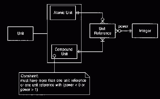
Figure 4 Compound units.
This model can be used for acceleration and similar phenomena

Example We can represent an area of 150 square yards by a quantity whose number is 150 and whose unit is a compound unit with one unit reference to feet with power 2.

A variation on this model takes advantage of representing mappings with bags. Unlike the usual sets, bags allow us to use an object more than once in a mapping, as shown in Figure 5. Bags are particularly useful when we have a relationship that has a single numeric attribute.

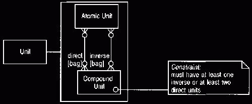
Figure 5 Compound units using bags.
This model is more compact than Figure 4

Example The acceleration due to gravity can be expressed as a quantity with number 9.81 and a compound unit with direct units of meter and inverse units of seconds and seconds.

The difference between Figures 4 and 5 is not great. There's a mild preference for Figure 5 because it avoids unit reference - a type that does not do much. The choice between these models does not matter to most clients of a compound unit. Only clients that need to break the compound unit down into atomic units are involved, and most of the type's clients would only need some printing representation.

4. Measurement

Modeling quantities as attributes may be useful for a single hospital department that collects a couple of dozen measurements for each in-patient visit.
However, when we look across all areas of medicine, we find thousands of potential measurements that could be made on one person.
Denning an attribute for each measurement would mean that one person could have thousands of operations--an untenably complex interface.
One solution is to consider all the various things that can be measured (height, weight, blood glucose level, and so on) as objects and to introduce the object type phenomenon type, as shown in Figure 6. A person would then have many measurements, each assigning a quantity to a specific phenomenon type.
The person would now have only one attribute for all measurements, and the complexity of dealing with the measurements would be shifted to
querying thousands of instances of measurement and phenomenon type. We could now add further attributes to the measurement to record such things as who did it, when it was done, where it was done, and so on.

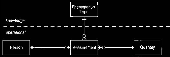
Figure 6 Introducing measurement and phenomenon type.
This model is useful if a large number of possible measurements would make person too complex.
The phenomenon types are things we know we can measure. Such knowledge is at the knowledge level of the model.

Example John Smith is 6 feet tall, which can be represented by a measurement whose person is John Smith, phenomenon type is height, and quantity is 6 feet.

Example John Smith has a peak expiratory flow rate (how much air can be blown out of the lungs, how fast) of 180 litres per minute.
This can be represented as a measurement whose person is John Smith, phenomenon type is peak expiratory flow rate, and quantity is 180 litres per minute.

Example A sample of concrete has a strength indicated by a force of 4000 pounds per square inch.
Here the person is replaced by a concrete sample with a measurement whose phenomenon type is strength and quantity is 4000 pounds per square inch.

This model has a simple division that was found to be very useful in later analysis. Measurements are created as part of the day-to-day operation of a system based on this model. Phenomenon types, however, are created on a much more infrequent basis because they represent the knowledge of what things to measure.
The two-level model was thus conceived: the operational level consists of the measurement, and the knowledge level consists of the phenomenon type.
Although it does not seem important in this simple example, we will see that thinking about these two levels is useful as we explore modeling more deeply.
(Although Figure 6 shows the dividing line, we have left it out of most of the following figures; however, we have a convention of drawing knowledge concepts toward the top of the figure.)

Modeling Principle The operational level has those concepts that change on a day-to-day basis.
Their configuration is constrained by a knowledge level that changes much less frequently.

Modeling Principle If a type has many, many similar associations, make all of these associations objects of a new type.
Create a knowledge level type to differentiate between them.

We could choose to add the unit of measurement to the phenomenon type and use numbers instead of quantities for the measurement. We prefer to keep quantities on the measurement so that we can easily support multiple units for a phenomenon type.
A set of units on a phenomenon type can be used to check the unit of an entered measurement and to provide a list for users to choose from.

5. Observation

Just as there are many quantitative statements we can make about a patient, there are also many important qualitative statements, such as gender, blood group, and whether or not they have diabetes. We cannot use attributes for these statements because there is such a large range of possibilities, so a construct similar to that for measurement is useful.

Consider the problem of recording a person's gender, which has two possible values: male and female. We can think of gender as being what we are measuring, and male and female are two values for it, just as any positive number is a meaningful value for the height of a person. We can then devise a new type, category observation, which is similar to measurement but has a category instead of quantity, as shown in Figure 7.
We can also devise another new type of observation that acts as a super-type to a measurement and a qualitative observation.

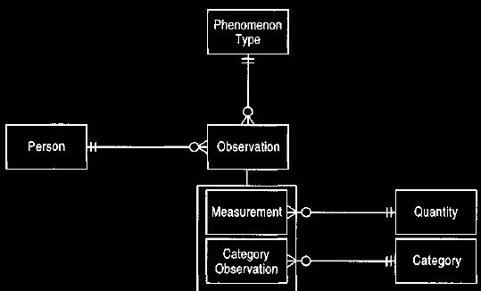
Figure 7 Observations and category observations.
This model supports qualitative measurements, such as blood group A.

Using Figure 7, we can say that gender is the instance of phenomenon type, and male and female are instances of category.
To record that a person is male, we create an observation with a category of male and a phenomenon type of gender.

We now have to consider how we can record that certain categories can be used only for certain phenomenon types. Tall, Average, and Short might be categories for the phenomenon type height, while A, B, A/B, and O might be categories for the phenomenon type blood group. This could be done by providing a relationship between category and phenomenon type. The interesting question then is the cardinality of the mapping from category to phenomenon type. We might ask, does the object A used in blood group potentially link to more than one phenomenon type? One answer is, of course it does: We grade liver function on the Childs-Pugh scale, which has values A (reasonable), B (moderate), and C (poor). This raises the question of what we mean by A. If we mean merely the string consisting of the character 'A,' then the mapping is multi-valued and the category is independent of the phenomenon type.
The category's meaning is only clear when a phenomenon type is brought in through a qualitative observation. The alternative is to make the mapping single-valued, where the category is only defined within the context of the phenomenon type; that is, it is not A but blood group A.

What difference is this to us? The single-valued case allows us to record useful information about the categories, such as A is better than B with respect to liver function, while no such ordering exists for blood groups.

Initial investigations of the clinical process reveals a common sequence: a patient comes to the facility, evidence is collected about the patient's condition, and a clinician makes an assessment. For example, a patient might come in complaining of excessive thirst, weight loss, and frequent urination (polyuria).
This would lead a clinician to diagnose diabetes. A couple of things are important about recording this diagnosis. First, it is not sufficient simply to note that the patient has diabetes; the clinician must also explicitly record the evidence used to come up with this diagnosis. Second, the clinician does not make this kind of deduction out of thin air. Random evidence is not assembled into random deductions. The clinician must rely on clinical knowledge.

Consider placing this process in the model we have so far. The patient is suffering from weight loss. We can capture this by saying that there is a phenomenon type of change in weight, with linked categories of gain, loss, and steady. Similarly there is a phenomenon type of diabetes with categories of present and absent.
Clearly we can record the link between the observations by placing a suitable recursive relationship on observation, as shown in Figure 8.
We can thus record the link between the observation of diabetes and its evidence. We also need to record the clinical knowledge of the link between weight loss and diabetes. Using the model shown in Figure 7, we would have difficulty recording this link. The phenomenon type of change in weight and the category of loss are only linked when an observation is made. We need a way to say that weight loss, which can exist without any observations, is at the knowledge level. Making the mapping from category to phenomenon type single-valued provides the way. (Section 11 discusses this further.)

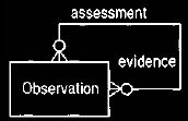
Figure 8 Recursive relationship to record evidence and assessment.

This was the compelling evidence for making the mapping from category to phenomenon type single-valued. It moved category to the knowledge level and renamed it phenomenon, as shown in Figure 9. Phenomena define the possible values for some phenomenon type.

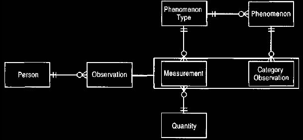
Figure 9 Phenomenon (formerly category) in the knowledge level.
Placing qualitative statements (such as blood group A) in the knowledge level allows them to be used in rules.

Example The fact that a person is blood group A is indicated by a category observation of a person whose phenomenon is blood group A.
The blood group A phenomenon is linked to the phenomenon type of blood group.

Example We can model a low oil level in a car as a category observation of the car. The phenomenon type is oil level with possible phenomena of over-full, OK, and low. The observation links the car to the low phenomenon.

The model in Figure 9 works well for category observations with several values for a phenomenon type. But many observations involve merely a statement of absence or presence rather than a range of values. Diseases are good examples of these: Diabetes is either present or absent. We could use Figure 9 with the phenomena diabetes absent and diabetes present. This ability to explicitly record the absence of diabetes is important, but it may also be sensible to record absence of weight loss. (If a patient comes in with symptoms of diabetes but has not been losing weight, then that would contra-indicate diabetes. This does not imply that the weight is increasing or steady, merely that it is not decreasing.) Indeed we can record the absence of any phenomenon, particularly to eliminate hypothetical diagnoses.
Thus the model shown in Figure 10 allows any category observation to have presence and absence. Observation concept is added as a super-type of phenomenon.
This is done to allow diabetes to be an observation concept without attaching it to some phenomenon type.

Example We record the fact that John Smith has diabetes by a presence observation of John Smith linked to the observation concept diabetes.

Example We represent spalling (deteriorating) concrete in a tunnel by an observation with the tunnel instead of the person, and an observation concept of spalling concrete. We also need a feature on the observation to indicate where in the tunnel the spalling occurs.
(Medical observations may also need an anatomical location for some observation concepts.)

6. Sub-typing Observation Concepts

Figure 10 introduces a super-type relationship that allows generalization of observation concepts. This is quite common in medicine and is valuable because observations can be made at any level of generality. If an observation is made of the presence of the sub-type, then all super-types are also considered to be present.
However, if an observation is made of the absence of a sub-type, then that implies neither presence nor absence of super-types. Observation of absence does imply all sub-types are also absent. Thus presence is propagated up the super-type hierarchy, while absence is propagated downward.

Example Diabetes is an observation concept with two sub-types: type I diabetes and type II diabetes. An observation that type I diabetes is present for John Smith implies that diabetes is also present for John Smith.

Example Blood group A is called polymorphic because it can be sub-typed to A1 and A2. The other blood groups are not polymorphic.

7. Protocol

An important knowledge concept for recording observations is the protocol-- the method by which the observations were made. We can measure a person's body temperature by placing a thermometer in the mouth, armpit, or rectum. Usually the temperature readings these techniques yield can be considered the same; nonetheless, it is vital to record which approach we used. A strange observation can often be explained by understanding the technique that was used to reach it.
Thus in health care it is accepted practice to always record what tests are used to record observations.

One of the values of a protocol is that it can be used to determine the accuracy and sensitivity of a measurement. This information could be recorded on the measurement itself, but usually it is based on the protocol that is used for the observation. Holding it at the protocol makes it easier to capture this information.

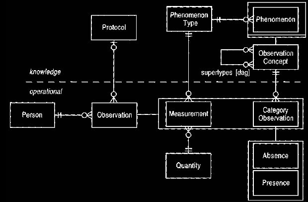
Figure 10 Absence and presence of observation concepts.
The absence of a phenomenon can be as valuable as finding a presence.

8. Dual Time Record

Observations often have a limited time period during which they can be applied. The end of the time period indicates when the observation is no longer applicable.
This time period is different than the time at which the observation is made. Thus there are two time records (which may be periods or single time points) for each observation: one to record when the observation is applicable and the second when it is recorded, as shown in Figure 11.

Example At a consultation on May 1, 2008, John Smith tells his doctor that he had chest pain six months ago that lasted for a week.
The doctor records this as an observation of the presence of the observation concept chest pain. The applicability time record is a time period starting at November 1, 2007 and ending at November 30, 2007. The recording time is the time-point May 1,2008. (Note that some way of recording approximate time-points would be valuable here.)

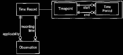
Figure 11 Dual time record for observation.
A time record allows both periods and single points to be recorded. Most events have a
separate occurring and recording time

9. Rejected Observation

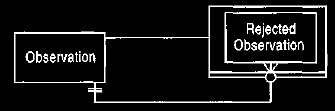
Figure 12 Rejected observations.
Observations cannot be deleted if a full audit trail is needed.

Example John Smith has a blood test that indicates a large mean corpuscular volume. This can be due to either pernicious anemia or alcohol abuse.
John Smith informs the doctor that he drinks very little alcohol. This indicates the presence of pernicious anemia, which leads to further tests and treatment.
Six months later it is discovered that John Smith drinks heavily. This information indicates that the observation of pernicious anemia should be
rejected by an observation of alcohol abuse. The rejected observation of pernicious anemia must be retained to explain the treatment that ensued.

10. Active Observation, Hypothesis, and Projection

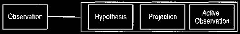
Figure 13 Active observation, hypothesis, and projection.

Example A patient with observations of the presence of thirst, weight loss, and polyuria indicates diabetes. With just these symptoms, however,
a clinician makes a hypothesis of diabetes and orders a measurement of the fasting blood glucose. The result of this test indicates whether to confirm the hypothesis or reject it.

Both sub-types, active observation and hypothesis, represent observations of the current state of the patient. Projections are observations that the clinician thinks might occur in the future. Often clinicians decide on treatments by considering future conditions that may occur. If the prediction is true, it is recorded with an additional active observation.

Example If a patient has rheumatic fever, or consequent rheumatic valve disease, there is a risk of endocarditis. This risk is recorded as a projection of endocarditis. Treatments will then be based on this projection.

The certainty of observations is one area of much discussion. The final model reflects the clinicians' views of what was the most natural.
The classic approach of assigning probabilities might make sense to science fiction aficionados, but it clearly did not to clinicians (who could predict asking questions such as "What are we to make of the difference between 0.8 and 0.7?"). With active observation and hypothesis, the final concept is more clear, although the choice of which classification to use is more problematic. In the end only the group of experienced clinicians can make a useful decision on this area in an almost instinctive way. The professional analyst can only point out some formal consequences.

11. Associated Observation

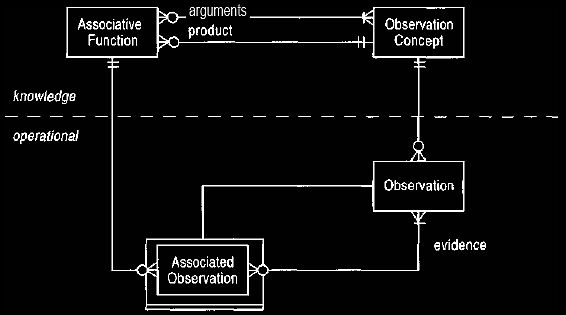
Figure 14 Links between observations.
Actual evidence chains for a patient are recorded at the operational level. The knowledge level describes what chains are possible.

Example A clinician observes weight loss, thirst, and polyuria in a patient and makes an associated observation (and hypothesis) of diabetes based on the evidence observations.
The associated observation is linked to an associative function whose arguments are the observation concepts--weight loss, thirst, and polyuria - and whose product is diabetes.

Example If our car does not start and the lights do not work, then both of these observations are evidence for the associated observation of a dead battery. Car not starting, lights not working, and dead battery are all observation concepts linked by an associative function.

Note that the knowledge and operational levels are not complete mirror images of each other. Associated observation is a sub-type of observation, but associative function is not a sub-type of observation concept. It seemed natural to make associated observation a sub-type of observation since, at the operational level, one particular observation is made with supporting evidence. At the knowledge level, the rule with arguments and conclusion is recorded. One observation concept may have several associative functions for which it is the result, but a particular observation has only one set of observations as evidence.

12. Process of Observation

This section has concentrated on the static elements of observation: what an observation or measurement is and how we can record it in a generic way to support the analysis that clinicians need to perform on it. It is significant that in modeling we found that we could conceive of a general static model, but the behavioral part was much more dependent on individual departments. Of course, a static model implies a great deal of behavior. Behaviors exist to create observations and to provide various ways of navigating associations to understand how those observations fit with other observations. The behavior we cannot imply, however, is the sequence of observations that a typical department makes. Often a clinician has some path of observations that can be taken. Departmental policy may be to record this path in terms of higher-level protocols (see Analysis of Planning of Business>).
It is difficult, and almost certainly impossible, to design a general process that all clinicians could use.
It is possible, however, to sketch an outline of the process involved in making observations. We begin by looking at how making a new observation can trigger further observations, as shown in Figure 15. Whenever clinicians make observations, they consider the possibility of other associated observations. They use the associative functions they know to come up with a list of possible observation concepts that might be associated with the triggering observations. They can then propose further observations as needed.

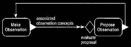
Figure 15 Making an observation triggers further observations.
Further observations are suggested by the knowledge level.

In Figure 15 the concurrent trigger rule is labelled "associated observation concepts." In event diagrams, trigger rules have two purposes. First, they show cause and effect. When we are considering business processes, this is usually enough, but as we delve deeper we see a second purpose. Any operation has input and output. The trigger that connects two operations must describe how to get from the output of the triggering operation to the input of the triggered operation.
In many cases this is trivial, as they are the same object (as in the trigger from propose observation to make observation shown in Figure 15). However they can get quite complex, as in finding associated observation concepts.

When we have a more complex trigger rule, we can represent the trigger rule with another event diagram. Figures 16 and 17 do this for the associated observation concepts trigger. We begin by finding all the associative functions whose input includes the initial observation's observation concept. We then evaluate each of these associative functions. For each one that evaluates to true, we find the product and add it to the answer. Since these event diagrams describe a trigger rule query, all the operations must be accessors and hence must not change the observable state of any object.

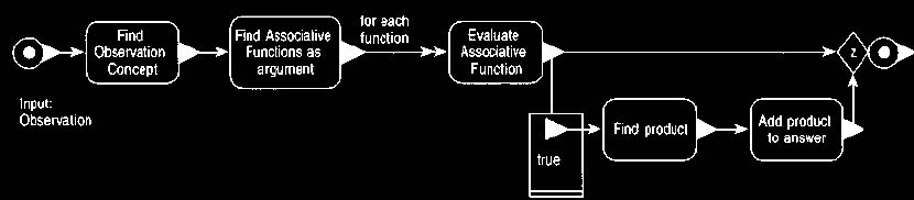
Figure 16 Event diagram to describe the query for finding associated observations. This lies on the concurrent trigger of Figure 15 or in the operation of Figure 18.

When the trigger rule query is complex, you can also represent the query as an operation in its own right, as shown in Figure 18. Either method is correct.

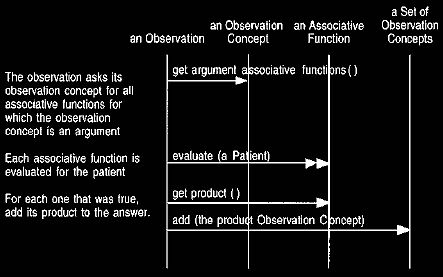
Figure 17 An interaction diagram for finding the possible observation concepts implied by an observation.
This interaction diagram supports Figure 16.

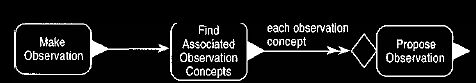
Figure 18 Notating the query explicitly as an operation.
This is equivalent to Figure 15. You can either show queries as operations or consider them part of the trigger, trading simplicity for compactness.

Even after the query, there is a control condition (evaluate proposal) before an observation is proposed. The query suggests possible observation concepts to look for based on the associative functions. This step could easily be done by software in a decision support system. The control condition represents the extra step of deciding whether the suggested observation concept is worth testing for. We did not feel we could formally model this process, implying that this step is beyond software and can only be done in the clinician's head.

Figure 19 includes additional triggers that arise from projections and active observations. The triggers to propose intervention work in a similar way to the previous case. We suggest interventions that are evaluated by the clinician before they are proposed. This reinforces the fact that although any observation can lead to further observations being made, only active observations or projections (not hypotheses) lead to interventions.
(An intervention is an action which either intends or risks a change in state of the patient.)
The trigger queries work in a similar way with the knowledge level but involve start functions, which are discussed briefly in Planning of Business, Section 7.

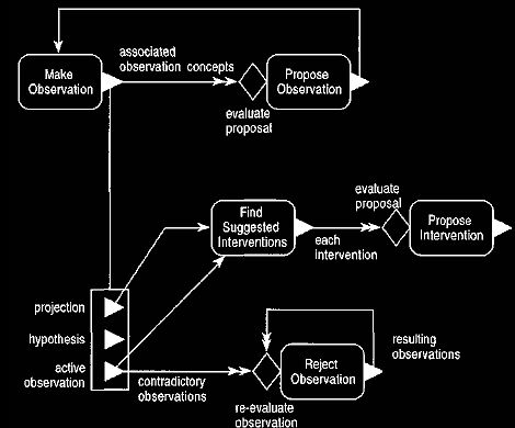
Figure 19 Event diagram for the process of working with observations. This extends Figure 15 with similar triggers for interventions and rejections.

The final trigger on Figure 19 shows how the appearance of an active observation can contradict other observations and thus lead to those observations
being rejected. Again this can involve associative functions, but this time we are looking for a contradiction. Once an observation (which may be a hypothesis) is rejected, further observations which were supported by this observation must be reconsidered.

One of the interesting things about the work that produced these patterns is the way the abstractions were found. Although the final results discussed here are usually structural, behavioral modeling played a central role in understanding how the concepts worked. The fact that clinicians did the modeling themselves was also crucial.
The abstraction of observation is central to these patterns; it ties together signs, symptoms, and diagnoses, which clinicians have long considered to be very different.
It was only by going through the modeling process that clinicians could pull out the abstraction.
If software engineers had come up with such an abstraction, we doubt if they could ever convince clinicians that it was valid.
And there would be good reason to be doubtful, since software engineers can never have that deep knowledge of medicine.
The best conceptual models are built by domain experts, and they are often the best conceptual modellers.